01What ERE is, and what the bench measures
Imagine shining a laser onto a solar cell. The laser's photons enter the material and hand their energy to electrons, lifting them into higher-energy states and leaving behind positively charged vacancies called holes. Together, an excited electron and the hole it left form an electron–hole pair.
Once created, those pairs recombine, and there are two ways it can go. In a radiative recombination event an electron fills a hole and releases the energy as a new photon. In a non-radiative one the energy is lost to defects, lattice vibrations and heat, and no light comes out at all.
A detector above the cell collects the light that escapes the device. That light is called photoluminescence, and measuring it is the whole job of this bench. Compare how much light the laser puts into the cell against how much comes back out, and you have the external radiative efficiency.
02Why ERE is worth measuring
ERE is a sensitive indicator of how much of a device is being lost to non-radiative recombination, and that loss has an electrical consequence. Reciprocity makes the connection explicit: a cell's open-circuit voltage falls below its radiative limit by the logarithm of its radiative efficiency.
That relation is what lets an optical measurement say something about a device's electrical quality. It does not make this a voltage measurement — the bench measures light, and the voltage figure is an inference drawn from it.
Why non-contact matters
The measurement needs no probes, no contacts and no fabrication step: light goes in, light comes out, and nothing touches the sample. That is what makes it useful partway through a process rather than only at the end of one.
A finished cell can be characterised electrically, but by then every step that could have gone wrong already has, and the wafer has absorbed the full cost of metallisation, patterning and packaging. Because ERE responds to the non-radiative recombination that defects and poor surfaces cause, it can be read off a bare wafer before any of that happens — which means a bad epitaxial layer or a badly passivated surface can be caught while the material is still cheap to throw away.
03How the bench works
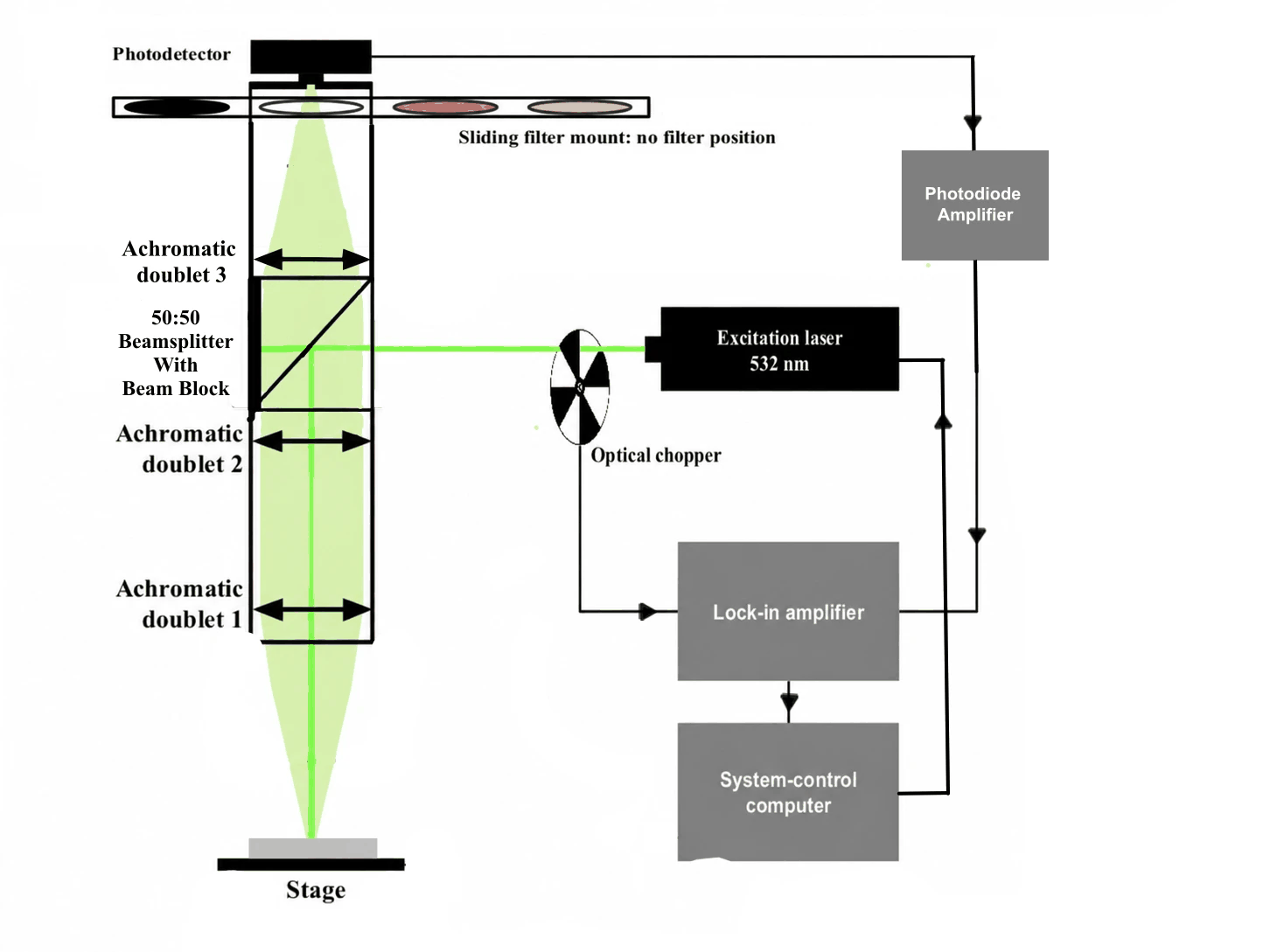
A 532 nm laser passes through an optical chopper, reflects off a 50:50 beamsplitter, and is focused down through two achromatic doublets onto the sample stage. Light coming back from the stage retraces that path, transmits through the beamsplitter, passes through a sliding four-position filter mount, and lands on a silicon photodiode. A transimpedance amplifier turns the photocurrent into a voltage, and a lock-in amplifier recovers the signal.
Why lock-in detection
The photoluminescence is a small signal arriving at a photodiode that also sees room light, mains hum and its own noise, so the bench moves the signal somewhere the noise is not. The chopper interrupts the pump at 191 Hz, which makes the photoluminescence switch on and off at 191 Hz while ambient light and amplifier offset do not. The chopper's reference output feeds the lock-in, which multiplies the incoming signal by that reference and integrates: anything not at the reference frequency averages toward zero. The frequency avoids harmonics of 60 Hz, since chopping at 180 or 240 Hz would drop the signal onto the strongest noise source in the building.
The lock-in reports an in-phase component X, a quadrature component Y, and the magnitude R. With the reference phase set correctly the whole signal sits in X and Y falls to nearly zero, so |Y|/|R| is a live check on whether the instrument is locked onto real signal or reporting noise — which section 06 uses.
Two measurements, divided
The bench never measures absolute photon flux, because it cannot. Instead it takes two measurements in the same optical path and divides them.
- Reference. A Spectralon diffuse reflector goes on the stage. It returns essentially all the 532 nm light that reaches it, so the detector voltage Vin is the "photons in" scale.
- Signal. The device goes on the stage and a long-pass filter drops in front of the detector, blocking the pump and passing the emission. The detector voltage Vout is the photoluminescence.
The ratio Vout/Vin is the raw measurement. Dividing is what makes the bench work: the laser power, the beamsplitter's reflectance and the fraction of light the collection lens happens to catch are all identical between the two readings, so they cancel and never have to be known. What is left is a number that is proportional to ERE but not yet equal to it, because the two paths are not quite symmetric. Section 05 is about closing that gap.
Why a Spectralon reference
For the cancellation to hold, the reference and the sample have to be collected with roughly the same efficiency. Spectralon is manufactured to be close to a Lambertian diffuser, and a planar semiconductor emitting through its surface is approximately Lambertian too, so the fraction of light the collection lens catches is similar for both. It is an approximation rather than an identity, and section 09 covers the second bench being built to do away with it.
Incident, not absorbed
This is the reason section 01 defined ERE against the light the laser delivers rather than the light the cell absorbs. The reference measurement sets the scale using the pump light arriving at the stage, and nothing in the two readings reveals how much of that light the device actually took in — so what comes out is ERE per incident photon. That makes it a property of the sample as a whole, material and geometry together, rather than a pure material property. Converting to the absorbed-photon definition would need a separate measurement of the sample's absorption at 532 nm, which this system does not do.
04What I inherited, and what I changed
The bench belonged to a master's student before me. I spent a short stretch in 2024 working alongside them on it and wrote some rudimentary automation for the system then. By the time I came back in 2026 they had left, someone had taken the bench apart, and it had never been brought to a state where the group could get usable numbers out of it.
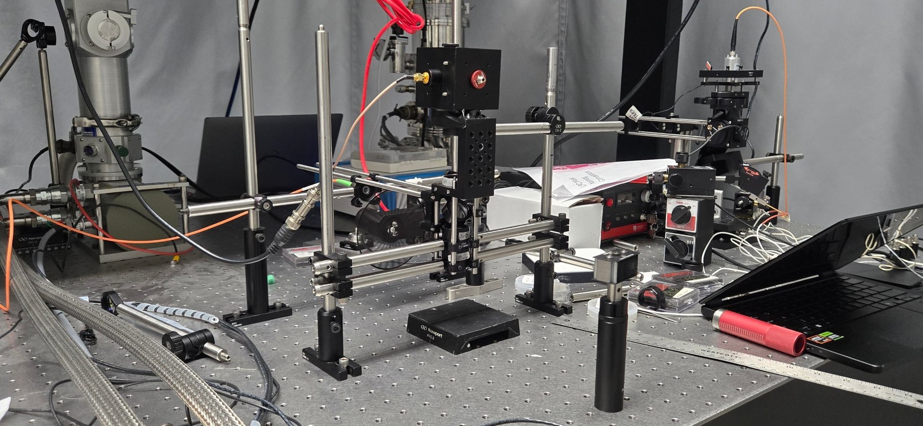
What I started with was roughly three photographs and a box of components, so the first job was reconstructing the system well enough to find out what was wrong with it. Quite a lot was.
Everything from here on is my own work: the rebuild and the optical changes below, the correction factor in section 05, the four control programs in section 06, the beam characterisation in section 08, and the results in between.
The filter was passing the pump
The most consequential find, and the one a photodiode could never have told me. A photodiode returns a single number and has no idea what wavelength produced it, so a filter that quietly passes the pump looks exactly like a device that emits well. Putting a spectrometer on the collection path instead splits that number out by wavelength, and the answer was immediate: the 532 nm pump line was still coming through, at a peak height roughly twice that of the emission band it was supposed to be blocked against.
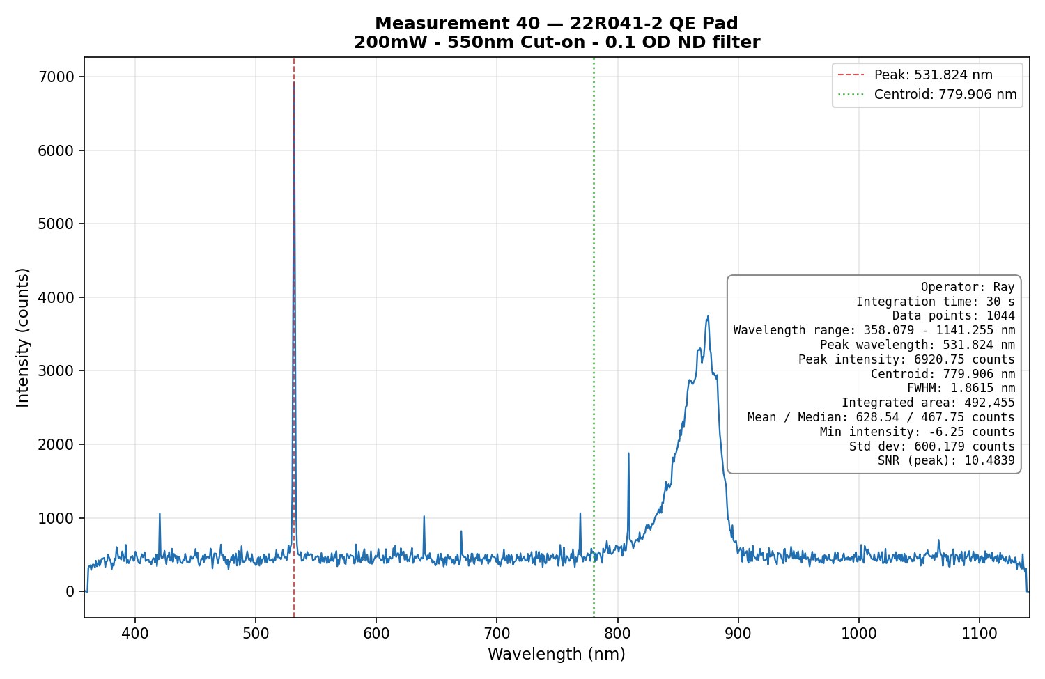
That is why nothing the bench had produced was usable. The correction in section 05 carries a term for exactly this contamination, and it only works while the leakage is small — a good long-pass blocker passes on the order of 10−5 of the pump. At the level in Fig. 3 it is not a correction any more; it is competing with the signal, and no arithmetic afterwards recovers the measurement.
Everything else
The filter was the find that mattered most, but it was not the only thing wrong. Reassembling the bench meant going through it optic by optic, and by the time it was producing numbers I trusted, most of the original hardware had been replaced or remounted. The changes below fall into two groups: things that were broken and had to go, and things that worked but made the measurement less repeatable than it needed to be.
| Change | Why |
|---|---|
| Replaced the emission filter | The inherited one leaked pump light at a level that dominated the signal |
| Replaced the beamsplitter | The inherited one was damaged and scattered light across the enclosure — an uncontrolled path to the detector that appears nowhere in the model |
| Moved the relay lenses from f₁+f₂ separation to as close together as possible | Less air path and fewer surfaces between the two elements for light to scatter off |
| New laser, and an optical chopper in place of direct modulation | Modulating a laser's drive current moves its power, wavelength and thermal state together, so laser drift lands at exactly the frequency the lock-in is looking for. A chopper leaves the laser running continuous-wave and modulates only the beam. |
| Rigid, non-adjustable beamsplitter mount | Repeatability — the cancellation in section 01 only holds if the geometry is genuinely identical between the two readings |
| Redesigned the laser input | The laser could previously shift in its mount, so it did not land on the same spot of the beamsplitter twice |
| Sent the sliding filter mount back to the manufacturer for repair | It failed mid-project |
05Deriving the correction factor
The raw ratio Vout/Vin is not ERE. Working out how far off it is means tracking optical power stage by stage down both paths and seeing what survives the division.
The two paths are not symmetric
This asymmetry is the whole result. In the reference measurement the light is at 532 nm for the entire round trip, so it crosses each lens twice at the same wavelength. In the signal measurement the pump goes down at 532 nm and the emission comes back at λemit, so each lens is crossed once at each wavelength.
Propagating power through every stage gives the reference reading
and the signal reading
Dividing, the laser power P0, the beamsplitter reflectance RBS and the collection fraction Ωcol cancel outright. The lens terms do not: the numerator carries one factor of each 532 nm transmission and the denominator carries two, so one survives underneath. What is left is a ratio of transmissions at the two wavelengths for every optic in the shared path. The absolute transmission of a lens never has to be known — only how much it changes between 532 nm and the emission wavelength.
Photons versus power
One correction has nothing to do with the optics. ERE is a ratio of photons, but what travels through the system and lands on the detector is power. Since E = hc/λ, converting between the two introduces λemit/λ532. For GaAs emitting near 870 nm under a 532 nm pump that is a factor of about 1.64 — not a rounding error, and a silent 60% bias if it is left out.
The leakage subtraction comes out for free
Some pump photons are never absorbed. They scatter off the sample, travel back up through the optics, and leak through the emission filter into Vout. Writing that contamination out stage by stage gives an expression identical to Vin except for a single factor, because the stray light follows exactly the same round-trip-at-532 nm geometry the reference measurement does. So the whole correction collapses to
The result
× (S532/Semit) × (λemit/λ532)
× (TBS,532/TBS,emit) × (T75,532/T75,emit) × (T150,532/T150,emit)
× 1/Tfilt,emit Detector responsivity ratio, photon-energy conversion, one transmission ratio per optic, and the filter's attenuation of the signal it exists to pass.
A Python tool evaluates that whole product from a pump wavelength and an emission wavelength. Every optical and detector curve is embedded as a lookup table transcribed from the manufacturer datasheets — photodiode responsivity, beamsplitter transmission, both achromat curves, the long-pass filter — with linear interpolation between tabulated points and an explicit warning when a request clamps at the end of a table. Nothing is read from disk at run time, so the tool cannot quietly return a wrong answer because a data file moved.
For the standard case — 532 nm pump, 870 nm GaAs emission — the correction factor comes out to 0.42. The raw voltage ratio overstates ERE by more than a factor of two.
One simplification is buried in all of that and worth naming. Every term with an emit subscript is evaluated at a single wavelength, as though the device emitted one colour. It does not — the emission in Fig. 3 is a band tens of nanometres wide, and each optic in the path transmits slightly differently across it. The correction uses the centre of that band and accepts the error, which is one thing I would like to change about the setup in the future
06Instrument control and the measurement workflow
When I worked at the bench in 2024, every measurement was taken manually. Setting up the lock-in amplifier correctly—adjusting the sensitivity range, setting the phase, and verifying that the signal was not overloading—required several minutes of front-panel work for each reading. The process had to be repeated at multiple laser powers.
A single ERE measurement requires both a Spectralon reference and a device measurement, repeated across several laser powers. As a result, obtaining one usable ERE result could take roughly half an hour of manual adjustments.
The process was also vulnerable to subtle errors that were not always obvious: a sensitivity range set one step too high, a phase that never fully stabilized, or an intermittent overload that went unnoticed. To address this, I wrote four programs that automate the measurement as extensively as possible. With the automated workflow, a measurement that once took about half an hour can now be completed in approximately three minutes.
The four programs
| Program | What it does |
|---|---|
| Lock-in recorder | The main acquisition tool. Live X/Y/R plot, checks and corrects overload, automatic phase correction, per-operator profiles, and CSV summaries alongside complete raw sample files |
| Measurement viewer | Reviews completed runs and verifies that the data were saved correctly before the sample is removed from the stage. |
| Filter-slider control | Finds the four-position filter slider on its own, homes it, and reconnects if the link drops. |
| Chopper control | Sets and reads the chopper frequency over RS-232 without requiring the operator to walk to the instrument. |
What a measurement looks like now
- Log in. The operator picks their profile, and the software pushes their saved instrument configuration — coupling, input, filter slope, notch filters, time constant, sensitivity — to the lock-in over GPIB. A status lamp confirms the chopper reference is locked before anything else happens.
- Reference. Spectralon on the stage, filter slider to the open position, laser power entered, and Begin Measurement. The software ranges the sensitivity, phases the lock-in, and starts recording.
- Collect. A live plot of X, Y and R runs at 5 Hz while samples accumulate. A hundred samples is the working minimum, then Finish & Save.
- Signal. Swap the Spectralon for the device, align the spot, send the filter slider home so the long-pass covers the detector, enter the device ID and notes, and run the same one-button cycle again.
- Check and analyse. The viewer confirms the run saved. The ratio of the two readings, multiplied by the correction factor from section 05, is the ERE.
How the automatic setup decides
Ranging and phasing were the biggest time sink in the manual workflow, so they are what step 2 above actually automates. Ranging means finding a sensitivity where the signal is large enough to resolve but not so large that the input stage clips. The routine runs in order:
- Drop to a fixed 100 ms time constant so every decision that follows is made on the same footing and settles quickly.
- Read the instrument status. If the reference is unlocked, stop immediately and name the chopper wiring — there is no point ranging a signal the lock-in is not locked to.
- If the input stage is clipping, reduce gain, or raise dynamic reserve once gain is exhausted. Deliberately leave the time constant alone: the output filter cannot fix input-stage clipping.
- If the output filter is overloading, raise the time constant instead — capped, so ranging never wanders off into multi-second settling.
- Read the signal as a fraction of full scale. If it is outside 12–60%, set the sensitivity directly at the value that puts it near 30%, rather than stepping toward it one notch at a time.
- Require three consecutive in-band readings before accepting the range, so a single lucky sample at a fluctuating input cannot pass.
- Set the measurement time constant — about sixty reference periods, snapped down to the instrument's discrete grid, which lands on 300 ms at 191 Hz and still does the right thing if the chopper frequency changes.
- Phase, then verify. Run the lock-in's auto-phase, then confirm |Y|/|R| ≤ 0.02 before accepting the result.
Perovskites are the one case that still wants a person. Their ERE changes while they are being measured, so the automatic loop — tuned for III-V devices that sit still — is switched off and gain and phase are set by hand.
None of this code is public. It was written for a working laboratory and is specific to the instruments on this bench, so what is on this page is a description of how it behaves rather than a repository link. I may be able to share it privately on request, if given approval.
07Results, and what they actually show
A bench that produces a number is not necessarily a bench that produces the right number. The first step, therefore, is to establish an independent prediction of the device’s expected external radiative efficiency (ERE).
Using reciprocity, the relation from Section 02 can be run backward. The device’s open-circuit voltage, VOC, is measured electrically, and the voltage it would have if every recombination event were radiative, VOC,ideal is calculated from detailed balance. The difference between these voltages determines the ERE:
Here, VOC,ideal is obtained from the radiative saturation current. That current is calculated by numerically integrating the blackbody photon flux above the device’s band gap and comparing it with the measured short-circuit current, Jsc.
The catch is where its inputs come from. Voc and Jsc are measured electrically, with the device under a solar simulator at one sun — so what reciprocity returns is not just an ERE, it is an ERE at one sun.
Measuring the beam
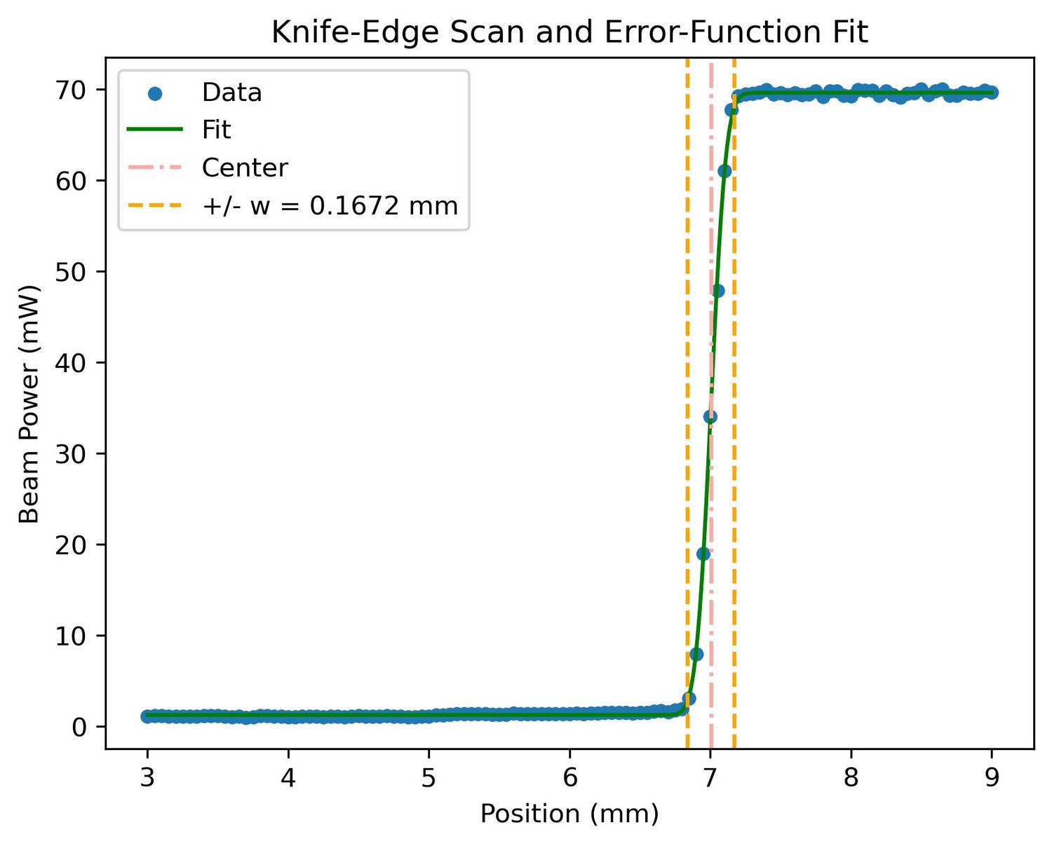
So what does one sun correspond to in terms of laser power on this bench? One sun is an irradiance of 100 mW/cm², and converting that irradiance into power requires knowing the area over which the beam is distributed. Therefore, the beam spot must be measured rather than relying on the power set on the laser. I measured the spot using a knife-edge scan, and got the results below:
Finding one sun on this beam
With that radius, one sun works out to about a quarter of a milliwatt at the laser:
Psample = 100 mW/cm2 × 8.783 × 10−4 cm2 = 0.0878 mW
Plaser = 0.0878 mW ÷ 0.346 = 0.254 mW Only 34.6% of the light dialled into the laser reaches the sample, most of it lost at the beamsplitter, so one sun at the device means about 0.25 mW at the source.
What the two methods give
Every point in Fig. 7 is a complete measurement in its own right — a Spectralon reference and a device reading, corrected and turned into an ERE — taken at a different laser power. ERE is not one number for a device: it climbs with excitation level, which is why the points trace a curve rather than a flat line, and why quoting an ERE without saying what illumination it was taken at means very little.
The points run from 5 to 15 mW because that is the range where the signal sits comfortably above the lock-in's noise floor. One sun is 0.254 mW, roughly twenty times lower than the weakest point that can be measured, so the value there cannot be read off the plot directly. Instead the curve is fitted to the points that can be taken and then evaluated at 0.254 mW — which is what the extrapolation down to the left-hand edge of the figure is doing.
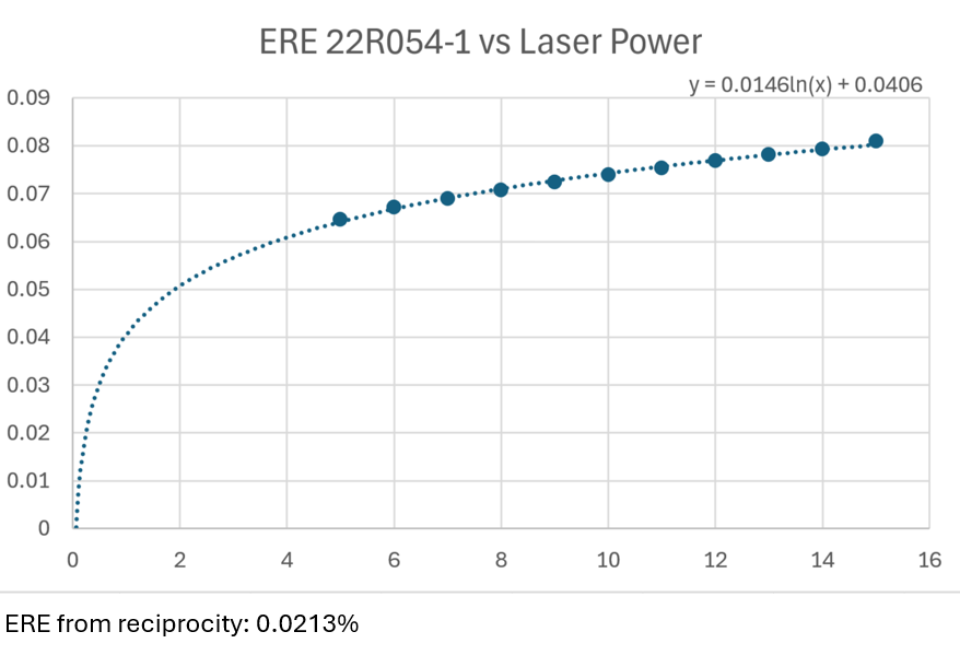
Evaluating the fit in Fig. 7 at 0.254 mW gives an ERE of 0.0206%. The reciprocity calculation on the same device gives 0.0213%. Those agree to within about three percent — one route optical, one route electrical, with no shared calibration between them.
Two things have to be said with equal weight. The fit is extrapolated down to roughly a twentieth of the lowest measured power, well outside the range the data actually covers. And the excitation spot is small enough that the result depends on where on the die it lands, so the closeness of this particular agreement owes something to positioning. It is a reason to keep going rather than a validation — but two independent methods landing this close is the strongest evidence the bench has produced that it is measuring the right thing.
08The one-sun problem
That last number came from extrapolating a curve rather than from a reading taken at one sun, and the obvious question is why not simply measure at 0.25 mW. The answer is that the beam is far too small, and everything below follows from that.
A radius of 0.167 mm puts the entire excitation inside a spot covering roughly 0.005% of the device pad — about one twenty-thousandth of it. The solar simulator that produced the reciprocity number floods the whole pad uniformly, so the two methods are not illuminating the same device even when they deliver the same irradiance to the patch they hit. Three consequences follow, and none of them can be fixed in software.
- The signal is too weak. One sun concentrated into a spot that small needs only about 0.25 mW, and the lock-in reads noise below roughly 5 mW for GaAs and about 1 mW for perovskites. One sun sits an order of magnitude beneath the floor, so it cannot be measured directly on either material.
- Current crowding. Carriers generated in one small region have to spread laterally to reach the contacts, giving an internal current distribution nothing like the one full-pad illumination produces — so even a reading taken at exactly the right irradiance is not measuring quite the same condition.
- Local non-uniformity. Devices are not spatially uniform, and PL mapping has shown older ones varying roughly fourfold across a single die. A spot this small lands on an unusually good or bad patch instead of sampling the device average, which is the positioning sensitivity that qualifies the agreement in section 07.
Matching irradiance alone would not settle it either, because the sun is broadband and a 532 nm laser is not. Equal irradiance does not mean equal carrier generation.
Ways out
Matching short-circuit current and open-circuit voltage against the solar simulator is the direct approach, and the simulator is already in the loop — it is where the reciprocity numbers in section 07 come from. What stops it is that the illuminated area has to be comparable between the two setups — a beam expanded to the size of the pad and flattened into a top hat, which needs beam-shaping optics costing thousands to tens of thousands of dollars.
The practical route is cross-calibration. Measure several samples on an independently calibrated ERE system at another university, bring them back, sweep laser power here, and find the power that reproduces the known one-sun result. That sidesteps having to prove the laser and the simulator are physically equivalent, and using several samples tests whether the calibration holds across devices rather than resting on one.
In the meantime the working method is the one behind Fig. 7 — start well above the noise floor, step upward, build the curve, and extrapolate down to 0.25 mW. Any one-sun figure obtained that way is an extrapolation rather than a measurement, and this page says so on purpose.
09What comes next
Two things are happening in parallel: one that makes this bench better at what it already does, and one that goes after the limit it can never clear.
Expanding the beam
For the bench as it stands, this is the change worth making. Nearly every limitation in section 08 traces back to a spot covering a twenty-thousandth of the device pad. Expanding the beam and trimming it with an iris does not make it a top hat — a Gaussian is still brighter in the middle than at the edges — but it makes the result far less sensitive to where the beam lands, brings more of the device into the measurement, and raises the total signal. That last part matters most: more signal means the usable range extends to lower powers, which shortens the extrapolation the one-sun number currently depends on.
A second bench, for absolute ERE
Section 07 explains why this system can only ever produce relative ERE: it has no radiometrically calibrated detector, and it never sees all the light the device emits. Both are properties of the geometry, so the answer is a different geometry. A second setup is being built to measure absolute ERE directly.
The device sits over a small pinhole in an integrating sphere, and the laser lives inside the sphere, illuminating the device through that pinhole. Everything the device emits back into the sphere is collected by the sphere itself rather than by a lens subtending some fraction of a hemisphere, and a spectrometer reads what the sphere collects.
That arrangement removes both limits at once. The collection fraction stops being an approximation — there is no longer a Spectralon reference standing in for the sample's angular distribution, because the sphere captures essentially all of it either way. And a spectrometer that has been calibrated against a known source reports absolute spectral irradiance rather than an arbitrary voltage, which is the other half of what an absolute measurement needs. Resolving wavelength is worth having on its own terms too: it is what caught the filter leak in Fig. 3, and it is why a leak could not hide on the new bench the way it hid on this one.
That project is a group effort rather than mine alone. My part in it has been calibrating the spectrometer and writing some of the data collection software.